Once I start shrinking, where do I stop???
The (overall) Optimal choice of Shrinkage m-Extent is quite simple when using the NEW (2021) Efficient Path.
However, for traditional 1- and 2-parameter Paths, this may well be THE question!!! This is why Shrinkage methods in Regression have been considered highly controversial for much of the last 40 years. A review of the history of Ridge Regression reveals "root causes" of Controversy...
Relatively widespread interest in ridge regression was initially sparked by Hoerl and Kennard(1970) when they suggested plotting the elements of their shrinkage estimator of regression beta-coefficients in a graphical display called the RIDGE TRACE. They observed that the relative magnitudes of the fitted coefficients tend to stabilize as shrinkage occurs. And they over-optimistically implied that it is "easy" to pick an extent of shrinkage, via visual examination of that coefficient trace, that achieves lower MSE risk than least squares.
Today, we know it just ain't easy. Even the relatively "tiny" amount of shrinkage that results using James-Stein-like estimators [Strawderman(1978), Casella(1981,1985)] when R-squared is large (greater than .8, say) is already "too much" to allow them to dominate least squares in any matrix-valued MSE risk sense. In other words, least squares is admissible in all meaningful (multivariate) senses [Brown(1975), Bunke(1975).]
Ok, so Hoerl-Kennard were wrong about guaranteed risk improvements. But, in the eyes of their major critics, this probably wasn't their BIG mistake! No, they were unabashedly telling regression practitioners to... LOOK AT THEIR DATA (via that trace display) ...before subjectively "picking" a solution. And all "purists" certainly consider any tactic like this a real NO! NO!
In all fairness, almost everybody does this sort of thing in one way or another. Regression practitioners are constantly being encouraged to actively explore many different potential models for their data. Some of these alternatives change the functional form of the model, drop relatively uninteresting variables, or set-aside relatively influential observations. But who tells those practitioners that it can be misleading to simply report the least squares estimates and confidence intervals for that final model as if it were the only model they ever even considered?
In other words, shrinkage/ridge methods have served as a convenient "whipping-boy" for all sorts of statistical practices that are questionable simply because they are based mainly upon heuristics.
My implementations of shrinkage/ridge regression algorithms skirt the above somewhat delicate issues by providing theoretically sound and objective (rather than subjective) criteria for deciding which path to follow and where to stop shrinking along that path. My algorithms use a normal-theory, maximum likelihood formulation to quantify the effects of shrinkage. Simulation studies suggest that my 2-parameter (Q-shape & M-extent) approach can work very, very well in practice [Gibbons(1981).]
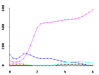
My shrinkage algorithms also display a wide spectrum of "trace" visualizations. For example, they display traces of scaled (relative) MSE risk estimates for individual coefficients...

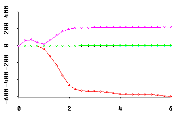
traces of "excess eigen-value" estimates (with at most one negative estimate)...

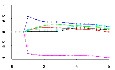
traces of "inferior direction cosine" estimates (for the one negative eigen-value above)...

and even traces of multiplicative shrinkage factors (not shown) as well as the more traditional traces of shrunken coefficients.
Note that the horizontal axis for all of these traces is the Multicollinearity Allowance parameter, 0 <= MCAL <= p. This MCAL can usually be interpreted as the approximate rank deficiency in the predictor variables X-matrix. Displays of fitted coefficients in least angle regression (LAR) use a horizontal axis scaling quite similar to MCAL!
Why should these trace displays be of interest to YOU? Because... OH!, WHAT A DATA ANALYTIC STORY THEY CAN TELL! In Obenchain(1980), I called this the "see power" of shrinkage in regression.
For explanations of (and interpretations for) these sorts of traces, see Obenchain(1984, 1995); for the underlying maximum-likelihood estimation theory, see Obenchain(1978).