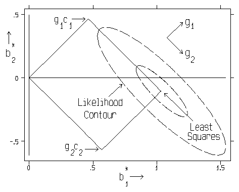
The following formulas describe the FORM and EXTENT of shrinkage yielding 2-parameter generalized ridge regression estimators.

Our first formula, above, represents the 2-parameter family using notation like that of Goldstein and Smith(1974). Here we have assumed that the response vector, y, and all p columns of the (nonconstant) regressors matrix, X, have been "centered" by subtracting off observed mean value from each of the n observations. Thus Rank(X) = r can exceed neither p nor (n-1).
Insight into the form of the shrinkage path that results as k increases (from zero to infinity) for a fixed value of Q is provided by the "singular value decomposition" of the regressor X matrix and the corresponding "eigenvalue decomposition" of X'X.

The H matrix above of "principal axis regressor coordinates" is (n by r) and semi-orthogonal (H'H = I.) And the G matrix of "principal axis direction cosines" is (p by r) and semi-orthogonal (G'G = I.) In the full-column-rank case (r = p), G is orthogonal; i.e. GG' is then also an identity matrix.
The (r by r) diagonal "Lambda" matrix above contains the ordered and strictly positive eigenvalues of X'X; Lambda(1) >= ... >= Lambda(r) > 0. Thus our operational rule for determining the Q-th power of X'X (where Q may not be an integer) will simply be to raise all of the positive eigenvalues of X'X to the Q-th power, pre-multiply by G, and post-multiply by G'.
Taken together, these decompositions allow us to recognize the above 2-parameter (k and Q) family of shrinkage estimators, beta-star, as being a special case of r-dimensional generalized ridge regression...

where the (r by r) diagonal "Delta" matrix contains the multiplicative shrinkage factors along the r principal axes of X. Each of these Delta(i) factors range from 0 to 1 (i = 1, 2, ..., r.) And the (r by 1) column vector, c, contains the uncorrelated components of the ordinary least squares estimate, beta-hat = G c, of the true regression coefficient beta vector. The variance matrix of c is the diagonal Lambda-inverse matrix times the scalar value of the error sigma-square.

In fact, we now see that the 2-parameter family of shrinkage estimators from our first equation, above, is the special case of the last equation in which...

Actually, the "k" parameter is not a very good measure of the extent of shrinkage in the sense that the sizes of all r shrinkage factors, Delta, can depend more on one's choice of Q than on one's choice of k. Specifically, the k-values corresponding to two different choices of Q are usually not comparable.
Thus my algorithms use the m = MCAL = "multicollinearity allowance" parameter of Obenchain and Vinod(1974) to index the M-extent of Shrinkage along paths. This parameter is defined as follows...

Note that the range of MCAL is finite; MCAL ranges from 0 to r=Rank(X), inclusive. Whatever may be your choice of Q-shape, the OLS solution always occurs at the beginning of the shrinkage path at MCAL=0 (k=0 and D=I) and the terminus of the shrinkage path, where the fitted regression hyperplane becomes "horizontal" (slope=0 in all p-directions of X space) and y-hat = y-bar, always occurs at MCAL = r ( k = +infinity and D = 0 ). RXridge.LSP uses Newtonian descent methods to compute the numerical value of k corresponding to given values of MCAL and Q-shape.
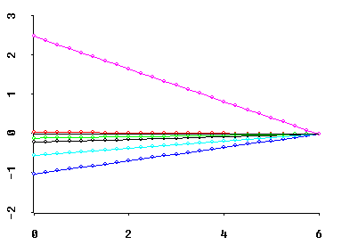
In addition to having finite (rather than infinite) range, MCAL has a large number of other advantages over k when used as the scaling for the horizontal axis of ridge TRACE displays. For example, shrunken regression coefficients with stable relative magnitudes form straight lines when plotted versus MCAL.

Similarly, the average value of all r shrinkage factors is (r-MCAL)/r, which is the Theil(1963) proportion of Bayesian posterior precision due to sample information (rather than to prior information.) And this proportion decreases linearly as MCAL increases.
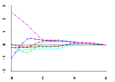
Perhaps most importantly, MCAL can frequently be interpreted as the approximate deficiency in the rank of X. For example, if a regressor X'X matrix has only two relatively small eigenvalues, then the coefficient ridge trace of best Q-shape typically "stabilizes" at about MCAL = 2. I.E., the coefficient trace then consists primarily of fairly straight lines between MCAL = 2 and MCAL = r = 6 in the graphic below.
