[1] Excluding the ICE Origin...
Since traditional approaches to ICE Statistical Inference use statistics derived from sample mean values of Cost and Effectiveness measures in random samples of patients, the (multivariate) Central Limit Theorem clearly applies, and the corresponding observed treatment differences clearly tend towards having a limiting Bivariate Normal Joint Distribution under rather weak regularity conditions. How come, then, are Normal-Theory Ellipsoidal Confidence Regions NOT routinely used in ICE Statistical Inference?
The "technical" answer to this question is that such a region could easily have (0, 0) as an Interior Point!. In fact, this sort of "problem" does occur in the "high uncertainty" numerical example from Obenchain(2008) and Obenchain, Robinson and Swindle(2005) that we are currently considering!
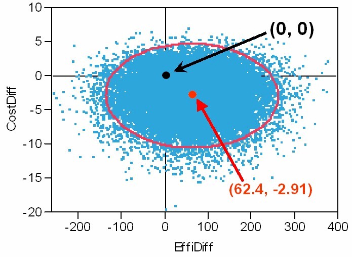
The Graphic below depicts: the ICE Origin at (0, 0),
the ICE Outcome Pair of Observed Effectiveness and Cost differences,
25K Re-samples from its Bootstrap Distribution of ICE Uncertainty,
and the resulting Normal-Theory 95% Confidence Ellipse.
The above Bootstrap Re-Sampled Distribution is somewhat skewed upwards
and has a somewhat long downwards, cost tail.
Clearly, this distribution is not "exactly" Bivariate Normal.
The observed (EffiDiff, CostDiff) correlation here is -0.0194.
What, then, might be the "conclusions" from the above sort of "Statistical Analysis"? I'm thinking they could sound quite grim and officious; i.e. something like the following... We conclude that there is no evidence of any true differences on Cost or Effectiveness between the new treatment T and our standard treatment S. Because all observed differences are NOT significantly different from zero, the new treatment option (T) will not be added to our formulary.
Thank goodness, published literature on Cost-Effectiveness Analysis has NOT endorsed use of the above sort of blatant "Hypothesis Testing" approach. In fact, in stark contrast with the above misleading "conclusions," it seems quite clear (at least to me) that the vast majority of re-sampled ICE outcomes in the above Bootstrap Distribution of ICE Uncertainty are more favorable to treatment T than to treatment S.
I have championed two different approaches that consistently provide more realistic answers to questions about Cost-Effectiveness Differences in Head-to-Head Treatment Comparisons than conventional "Significance Testing" possibly could!
[1] The Wedge-Shaped Confidence Regions described and depicted on my ICE Introduction page consistently exclude the ICE Origin. In fact, by insisting that (0, 0) be at most a Limit Point (and never an Interior Point) of the confidence region, Attention is much more clearly focused upon identifying Potential TRUE Differences between treatments ...either overall or in identifying relevant patient subgroups of differential responders.
[2] The ICE Quadrant Confidence Levels approach described in Obenchain, Robinson and Swindle(2005) is quite easy to understand and explain to statistical novices. By defining three progressive "levels" of ICE Statistical Dominance (Some, Much and Strict), this simple but Relatively Powerful and Discriminating Approach has several Theoretical and Practical Advantages. For example, in the above numerical example, the observed ICE Quadrant Confidence Levels are: SE => 64.4%, NE => 13.6%, SW => 18.1%, and NW => only 3.9%. In other words,
One's confidence that T is BOTH Less Costly AND More Effective than S is 64.4%.
One's confidence that T is EITHER Less Costly OR More Effective than S is 96.1%.
Thus our
Bootstrap ICE Quadrant Analysis shows that
T clearly expresses SOME
DOMINANCE over S and is on the borderline of expressing
MUCH DOMINANCE over S.