My statistical perspective on methods for ICE inference is that they address a fundamentally two-dimensional problem. In fact, I believe that ICE inference represents the single, most important and challenging area for practical application of basic concepts from multivariate analysis in health care today.
Introduction to Key Topics in ICE Graphical Perception and Interpretation:
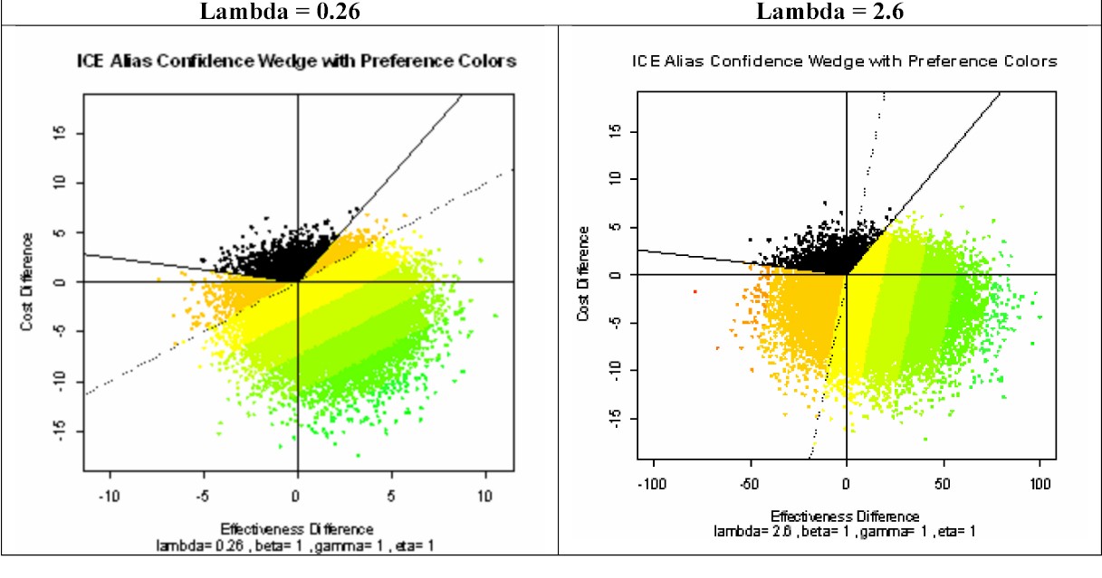
The above pair of graphical displays can be generated using the ICEwedge( ) and ICEcolor( ) functions contained within my ICEinfer R-package. The two graphs above show essentially the "same" Bootstrap Count-Outwards Wedge-Shaped 95% Confidence Region for the high-uncertainty numerical example of Obenchain(2008) and Obenchain, Robinson and Swindle(2005.) Due to high-uncertainty, this statistical region has an incredibly wide central-polar-angle of 237.o In other words, this particular confidence "wedge" is actually more than half of the whole bootstrap resampling pie! Yet, this 95% confidence region is at least somewhat restrictive in the sense that it spans only 66% (237 out of 360-degrees) of the total ICE plane.
Mathematically, the approach to defining a statistical confidence region illustrated here is said to be "equivariant" under changes in the Shadow Price of Health, usually denoted by the Greek symbol Lambda. Here, outcomes for the two numerical values of 0.26 and 2.6 are illustrated and compared. Technically, equivariance means that the operations of [a] changing Lambda and [b] forming the confidence wedge are commutative. One gets the same final wedge either when performing operation [b] then [a] or when performing operation [a] first and only then [b].
Actually, the above graphs (somewhat cunningly) use the so-called "alias" perspective (quite commonly used in both physics and computer science) where the bootstrap re-sampling scatter literally appears to be essentially unchanged between the left-hand and right-hand panels. However, because Lambda increases by a factor of ten in the second analysis, note that the scale changes along the horizontal axis (effectiveness in cost units); the left-hand effectiveness range of (-10 to +10) becomes (-100 to +100) in the right-hand graphic. Another difference that may emerge only upon quite careful examination of the above graphics is that (due to differences in R's initial random-number-generator "seed" value specified in two consecutive but separate analyses) the two scatters actually are not exactly identical! Still, up to this point in our discussion of the above graphics, there really are no important differences between them.
And now, the Kicker!!! When the bootstrap resampled outcomes within the above confidence wedges get COLORED with somewhat contradictory linear NB preferences (Beta = Gamma = Eta = 1) implied by two very different numerical values for Lambda, considerable additional economic variation (uncertainty) gets injected into the "Are there Differences?" question. See discussion Topic Two below for more information on this pivotal complication!
Topic One: Why Attempt to Exclude (0, 0)?
Topic Two: Two Sources of ICE Uncertainty
Topic Three: ICE Angle Serendipity
Topic Four: ICE Fieller's Theorem Wedges
Topic Five: ICE Preference Axioms
Topic Six: Variation in Willingness-to-Pay/Accept
Topic Seven: Eliminating Bias in Acceptability Curves