[4] Fieller's Theorem:
the "original" Wedge-Shaped ICE Confidence Region
Asymptotic Bivariate Normality of ICE Differences
Again, because ICE Inference is based upon sample mean values
in Cost and
Effectiveness measures, the (multivariate)
Central Limit Theorem clearly
applies, and the corresponding ICE Differences clearly tend towards having a
limiting Bivariate Normal Joint Distribution
under rather weak regularity conditions. Because this assumption of
normality is frequently quite realistic, it is extremely
natural to use the Fieller(1954) theorem
to develop confidence limits for the unknown, true ICE Ratio,
(CostDiff divided by EffeDiff).
Naturally, these intervals and the corresponding
BOW-TIE Shaped
confidence regions are very different
geometrically (and visually) from the much better-known,
elliptical regions needed to "cover" the unknown, true
ICE Outcome
PAIR, (EffeDiff,
CostDiff) with stated
confidence!
Application of Fieller's Theorem in
ICE Inference
Chaudhary and Stearns (1996) is an important
publication in ICE literature primarily because they displayed a closed-form
expression for computing the
Fieller Confidence Interval ...and its corresponding
BOW-TIE Shaped, bivariate confidence region. Earlier
papers by
OBrien, Willan and others
had explored various, simple Taylors series expansion approximations.
Practical Problems in
interpreting Confidence Intervals (Regions) from Fieller's Theorem
[a] Small Numerical Differences really are Rather
Un-Important!
Consider the following numerical example:
Fiellers Theorem 95%
Interval: -1.7652, +0.3463
ICE Angle Order Statistic
95% Interval: -1.7834, +0.3737
When "too many" decimal places are reported (as in the above
numerical listings), the Fieller Interval may
appear to be "different" from that of the corresponding Bootstrap
ICE Angle Interval. However, the graphical display below of the
corresponding 2-dimensional Confidence Regions
clearly shows that the Fieller and Bootstrap approaches
can be essentially equivalent in many cases...
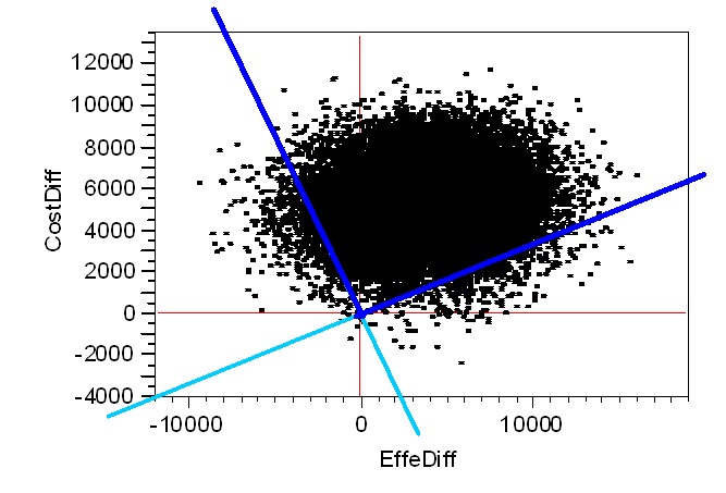
[b] Problematic "BOW-TIE" Shape:
Which "Half" should be
Thrown Away?
In the above graphic, the "top half" of the
Fieller BOW-TIE (that spans parts of the North-West and North-East ICE
Quadrants) is clearly the part to "keep." After all, this
particular "wedge" contains not only the ICE Outcome Pair, (+1,900, +5,289), of Observed
(Effectiveness, Cost) Differences but also roughly 95% of the Bootstrap
Re-sampled Outcomes! The "bottom half" (that
spans parts of the South-West and South-East ICE Quadrants) has the same
(finite, polar angular) size but contains almost no
Bootstrap Re-sampled Outcomes. And the two remaining wedges each contains
only roughly 2.5% of the Bootstrap Re-sampled Outcomes.
In summary, it usually is rather easy to decide which parts of the
Fieller BOW-TIE to throw away and ,thus, which
single
WEDGE to KEEP!
Still this sort of additional processing is a (mild) hassle
in the sense that it always needs to be done!
[c] "Infinite Intervals" can Result!
In fact, this phenomenon occurred in the above
example! The Fieller Interval (as well as the corresponding ICE
Angle Interval) contain all ICE Rays with Negative Slopes in the North-West
Quadrant that are numerically smaller (more negative) than roughly -1.77 as well as all
ICE Rays with Positive Slopes in the North-East Quadrant that are numerically larger
(more positive) than roughly +0.35. In other words, both the
Fieller and Bootstrap
intervals for this example can be described as consisting of the half-open interval (minus
infinity, -1.77] plus the half-open interval
[+0.35, plus infinity) ...with both parts being infinite
in length!
I really do not know why several ICE Confidence Interval
"critics" have tried to make such a BIG DEAL out of
this phenomenon. The reality is that ICE Ratios (Slopes) have a
simple discontinuity along the Vertical (EffeDiff=0) Axis
...where they suddenly jump between plus infinity and minus infinity.
My advise is this: Do not freak-out novices by reporting
these sorts of Intervals numerically; again, simply display the corresponding
Confidence Region graphically!
[d] Fieller's Theorem "Explodes" in High Uncertainty Cases!
Oh, Oh! This really is a MAJOR
SHORTCOMING. In fact, this is the ONLY REASON why the
Bootstrap Re-sampling approach using ICE Angle
Order Statistics should be considered to be more stable, robust and realistic than
the Fieller's Theorem approach!
By the way, it's rather obvious what goes "WRONG" with the
Fieller BOW-TIE in these "high uncertainty" cases. Each of the
opposing wedge-shaped "halves" of the BOW-TIE are
of the same (angular) size, so neither half can be wider
than 180-degrees!!! Thus, as the ICE Radius of the center-point of
the Bootstrap Re-sampling scatter decreases and the scatter approaches (and its
Convex-Hull ultimately covers) the ICE Origin, (0, 0), the
Fieller BOW-TIE WIDENS and eventually
attempts to COVER the entire ICE Plane.
Technically, the quantity within the square-root in the closed-form expression
of
Chaudhary and Stearns (1996) then becomes
NEGATIVE, and the only corresponding "solutions" for Fieller Confidence Limits become IMAGINARY!
In stark contrast, this sort of "explosion" simply cannot happen in the
Bootstrap Re-sampling approach using
ICE Angle Order Statistics because the
Central Polar Angle of the Bootstrap Wedge can easily exceed
180-degrees! In fact, the example wedge displayed on our
very first ICE Tutorial Page had a
Central Polar Angle spanning 237-degrees (i.e.
considerably more
than HALF of the full Bootstrap Re-sampling "PIE.")
Misconceptions that have lead to
Highly Questionable Simulation
Results
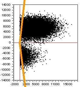
[a] Meaningless "Order Statistics" can result from
sorting ICE
Ratios instead of ICE Angles
The following is a computational "blunder" that I have seen
being repeated over and over again (in both ICE applications and ICE simulation
studies.) It's simply not appropriate (and
can be incredibly misleading and biased) to
(i) calculate the ICE Ratio for each Bootstrap Re-sample Outcome, to then (ii) sort these
values from numerically largest (most positive) to numerically smallest (most
negative), and finally (iii) to form a 95% Interval by "Counting Inwards"
2.5% of these ICE Ratio Order Statistics from each supposed "end" of the
resulting distribution.
This faulty algorithm essentially makes the incredibly
naive assumption, (depicted visually below) that all Bootstrap Re-sampled
Outcomes always have an observed
EffeDiff that is non-negative!
LOOK how "distorted" and "disjointed" the actual Bootstrap Distribution
(depicted above) becomes due to this blunder ...and how
LARGE and incredibly BIASED this blunder can make the resulting ICE Ratio
confidence wedge!!!
ICE Ratio Order Statistic
Interval: +12.4343, -12.458
In my opinion, all published simulation studies that claim that
bootstrap ICE intervals are "biased" (or have
"inferior" coverage) relative to Fieller ICE intervals
make this same, incredibly naive computational mistake.
[b] The ICE Ray with the Most Positive ICE Slope does not
necessarily correspond to the Upper (Counter-Clockwise) Confidence Limit
We also saw this phenomenon in the above numerical
example! The correct Counter-Clockwise (Upper) Confidence Limit was
the negative value (of -1.77 or -1.78 within the SW Quadrant) rather than the
positive value (of +0.35 or +0.37 within the NE Quadrant.)
[c] Incorrect or Misinterpreted Trignometric Formulas
I think that the simulation
results reported in Cook and Heyse (2000) are credible; anyway, they do agree
with what I have found in my own ICE experience. On the other hand, one of
their formulas does not give correct answers in any computing environment that I
have tried it in:
Theta (degrees) = 180*atan(DelCost/DelEffe)/pi
+ 180 when DelCost is negative
Unfortunately,
Fan and Zhou (2007) apparently
trusted this formula and (not surprisingly) got simulation results that conflict
with those of Cook and Heyse (2000)!!!
The following alternative formula gives correct answers in the "R"
environment:
Theta (degrees) = 180*atan(DelCost/DelEffe)/pi
+ 180 when DelCost is negative
+ 180 when DelEffe * DelCost is negative
The JMP (from SAS) environment returns a "missing value" when asked to
compute atan(1/0) and atan(-1/0).
WARNING: Obenchain manuscripts
emphasize the ICE Preference Symmetry Axiom and, thus, place the ICE Angle
Origin (Theta = 0) along the x = -y diagonal within the SE ICE Quadrant.
Correspondingly, I also restrict attention to the finite ICE Angle range of
(-180, +180] degrees. Cook and Heyse (2000) place their Theta origin at my
Theta = +45 degrees. Furthermore, they essentially use the "positive"
Theta range of [0, 360) degrees.
Summary
ICE Inference practitioners really do need to be
discouraged from using computing algorithms that have
not been validated.
If nothing else, a suite of benchmark numerical examples and corresponding
"correct" analyzes needs to be established to speed testing of all
new/alternative algorithms.
Furthermore, consensus on what (objectively) really are the relative strengths and weaknesses
of alternative ICE methodologies is quite badly needed. My very first ICE
communication (1997) called for collaboration on these vital sorts of "issues and
algorithms."
References:
Fieller EC. Some problems in interval
estimation. J R Stat Soc B 1954;
16, 175-183.
OBrien BJ, Drummond MF, Labelle RJ, Willan A.
In search of power and significance: issues in the design and analysis of
stochastic cost-effectiveness studies in health care. Med Care
1994; 32:
150-163.
Willan AR, O'Brien BJ. Confidence intervals for
cost-effectiveness ratios: an application of Fieller's theorem. Health
Economics 1996; 5:297-305.
Stinnett AA. Adjusting for bias in C=E ratio
estimates. Health Economics 1996; 5:470-472.
Chaudhary MA, Stearns SC. Estimating confidence
intervals for cost-effectiveness ratios: an example from a randomized trial.
Stat Med 1996; 15: 1447-1458.
Laska EM, Meisner M, Siegel C. Statistical inference
for cost-effectiveness ratios. Health
Economics 1997; 6: 229-242.
Polsky D, Glick HA, Willke R, Schulman K.
Confidence intervals for cost-effectiveness ratios: a comparison of four
methods. Health Economics 1997;
6: 243-252.
Tambour M, Zethraeus N. Bootstrap confidence intervals for
cost-effectiveness ratios: some simulation results. Health Economics
1998; 7:143-147.
Briggs AH, Fenn
P. Confidence intervals or surfaces? Uncertainty on the cost-effectiveness
plane (Student Corner.) Health Economics 1998; 7: 723-740.
Briggs AH, Mooney CZ, Wonderling DE.
Constructing confidence intervals for cost-effectiveness ratios: an evaluation
of parametric and non-parametric techniques using Monte Carlo simulation.
Stat Med 1999; 18:
3245-3262.
Cook JR, Heyse JF.
Use of an angular transformation
for ratio estimation in cost-effectiveness analysis. Stat Med
2000; 19: 2989-3003.
Jiang G, Wu J, Williams GR. Fiellers
interval and the bootstrap-fieller interval for the incremental
cost-effectiveness ratio. Health Serv Outcomes Res Method
2000; 1:
291-303.
Fan MY, Zhou XH. A simulation study to compare
methods for constructing confidence intervals
for the incremental cost-effectiveness ratio. Health Serv Outcomes Res
Method 2007; 7: 57-77.