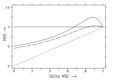
What does a Risk Profile for Maximum Likelihood Shrinkage typically look like?
The figure below is a plot of simulated Mean-Squared-Error RISK profiles for two maximum likelihood estimators over the full range of potential, optimal extents of shrinkage. In other words, the plot below depicts situations where the unknown, true MSE optimal shrinkage factor for a single regression coefficient ranges all of the way from 0 to 1.
Shrinking a coefficient all of the way to zero is optimal (Delta-MSE=0) when either the unknown, true value of that coefficient is zero or else in the limit as the error variance approaches +infinity. This is the LEFT-hand extreme in the plot below.
No shrinking at all is optimal (Delta-MSE=1) when either the error variance is zero or else in the limit as the unknown, true value of that coefficient approaches +infinity or -infinity. This is the RIGHT-hand extreme in the plot below.

The horizontal line in the above plot (constant risk normalized to equal one) represents the MSE of ordinary least squares (OLS). There is no real need to simulate a risk profile for OLS; OLS is well known to be the essentially unique, minimax rule.
The diagonal, dotted line in the above plot (from Risk=0 at Delta-MSE=0 to Risk=1 at Delta-MSE=1) represents the theoretical lower bound on MSE that would result if it were possible to always apply the exactly correct extent of shrinkage.
Of the two curves in the above plot, the top, solid curve is for the unrestricted maximum likelihood shrinkage of a single coefficient under normal distribution theory when the degrees-of-freedom for error equal 5. Note that MSE may decrease here by as much as 50% but never increases by more than 25%.
The lower, dashed curve in the above plot is for maximum likelihood, equal shrinkage of a pair of coefficients in the "null" case where their unknown, true values actually are equal. This second curve is also simulated under normal distribution theory when the degrees-of- freedom-for-error equal 5. Here MSE may decrease by more than 50% and yet never increases by more than only 6%.
See Obenchain(1997a) for more information about the above plot. Highly portable C-language source code and an MS-DOS executable for shrinkage risk simulation are also available for download from this web site.
Nav: Back