The RXridge algorithms for XLISP-Stat display two very different types of plots that display the potential effects of INFLUENTIAL OBSERVATIONS on model fits. Specifically, an observation can be influential because it has an outlying response value or because it represents a high leverage regressor combination ...or even for both reasons!
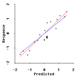
The first type of influence plot shows the observed response values, Y, vertically against their "standardized" predicted values along the horizontal axis. Since predictions are always linear combinations of the given regressor coordinates, the horizontal axis is best viewed as giving coordinates for a single, standardized composite regressor variable, x-star, that depends only upon the ORIENTATION of the shrinkage regression beta-star vector in p-dimensional space. The LENGTH of the shrinkage beta-star vector determines only the slope of the line on the Y versus x-star plot that represents the shrinkage fit.

The plot above corresponds to rather extreme shrinkage of the Longley data (p=6) to MCAL=5 along the Q= -1.5 path. The BLUE line represents this shrinkage fit while the RED line shows the "Visual Re-Regression" of Y onto the standardized x-star coordinates. Since the RED line is a clearly better fit here than the BLUE line, we see that this MCAL=5 extent of shrinkage is excessive.
The user of RXridge.LSP can use the MCAL slider control to reduce the shrinkage extent back to the MCAL=1.0 to 1.33 range to verify that the BLUE Q-shape= -1.5 fit is virtually identical to the RED VRR fit in this range.
Outliers show in this plot as large residuals ...i.e. these response Y values represent relatively large deviations from the fitted BLUE shrinkage line.
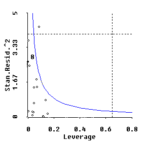
And the points with highest leverage along the 1-dimensional, composite x-star axis are the points toward the extreme left-hand and right-hand ends of the plot. Unfortunately, considerable information can be lost in attempting to display p-dimensional leverage information in one dimension. Anyway, these x-star axis leverages can be somewhat misleading. So, linked to the first plot, RXridge.LSP also displays a second plot of standardized residuals and p-dimensional leverages!
This second plot shows squared, standardized residuals (i.e. corrected for any differences in variance), vertically, against its p-dimensional regressor leverage ratio (prediction variance divided by residual variance) along the horizontal axis.

The Cook(1977) measure of overall influence for each observation is proportion to the product of its squared, standardized residual times its leverage ratio. Each contour of constant overall influence thus display as a hyperbola on our second type of plot. And this hyperbola can be moved either outward or inward using the overall "influence" slider control.